Sell In May Depends On Trend

Like it or not, “Sell in May and go away” is a Wall Street lore that just refuses to go away. Also known as the “Halloween Indicator”, the adage nowadays refers to owning equities for the six consecutive months from November through April, and being out of the stock market from May through October. Are the benefits, assuming there were any, valid today? Will selling in May really improve your equity portfolio’s performance?

Print PDF

“The difference in calendar year returns by selling in May is this: You have a 60% chance of underperforming, but in return for less volatility. “

At Coherent, we have been conducting our own research and analysis on the effects of seasonality on stock market performance using several databases tracing over 100-years. Our research is intended to answer many seasonality related questions in a rational and objective manner. We also gain insight from bona fide studies performed by others, after we have carefully read, verified, and understood the assumptions and the methodology behind their research.

Enjoy the video version of this article from our YouTube channel…

Synopsis

There is a statistically significant difference in calendar year returns between selling in May and holding all months, and it is this: You have a 60% chance of underperforming, but in return for less volatility.

Selling in May can be a significant benefit to the investor in market down-trends, but then it’s not about selling in May anymore. Investing has always depended on knowing what is the trend now, and what is its likelihood of changing in the near term.

So much written about selling in May is simply a regurgitation of other people’s studies or opinion, often without the benefit of their insight. Veritable studies stem from genuine curiosity and follow the scientific method. Authors have the prerogative to define their assumptions and methodologies which in turn can impact conclusions.

Sometimes, the best approach to answering a simple question is itself simple. We want to provide some rational and objective data behind the question of selling in May as it really matters to our clients.

1. Does selling in May produce different results?
2. If so, is the difference attributable to the market’s trend?
3. How would my portfolio have performed if I sat in cash May through October?
4. What’s the bottom line?

Our methodology is described in the footnotes.

Question #1: Does Selling In May Produce Different Results?

Let’s restate this question in a more specific and objectively provable manner. Is there a statistically significant difference in average calendar year returns over a given sample period, comparing being in cash from May through October to being in the market all year?

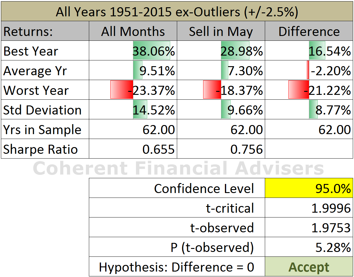
Using the classical approach, our hypothesis test found that the average difference in calendar year returns is not statistically different than zero within the standard 95% confidence interval. At face value, we would fail to reject (accept)¹ the null or no-difference hypothesis. However, upon closer examination, we note three important outcomes from this hypothesis test evident in figure-2.

First important outcome: If there is no difference in returns, the probability that the difference would be as large as 2.2% per year is only 5.28% according to the P-value. In my opinion, a 5-in-100 chance of a false positive is low enough to safely reject the no-difference hypothesis for its alternate – there is a difference.

Second important outcome: A portfolio which went to cash during May through October underperformed on average by 2.2% per year compared with holding all months. There is a difference, and the difference is NEGATIVE!

Third important outcome: The Sharpe ratio for the sell in May portfolio is 15% higher than for holding all months. The portfolio gave up 23% in average annual return, but 33% in volatility or standard deviation of return. The sell in May scenario has benefits appertaining to risk-adjusted return.

Question #2: Is The Difference Attributable To The Market’s Trend?

Yes, most definitely. The box and whiskers plot (figure-3) helps to visualize the returns distribution for holding all months compared with selling in May. We demarcated the data for calendar years in which returns were up, down, and flat.

When the market is down, one would expect to lose less by being on the sidelines for half of the year, especially when that half includes June and September. Our seasonality study shows that these two months return the worst performance of the twelve. But selling in May also misses four months of positive average returns, hence underperforming in up years. Our hypothesis test confirms our box plot observations as shown in the following table (figure-4).

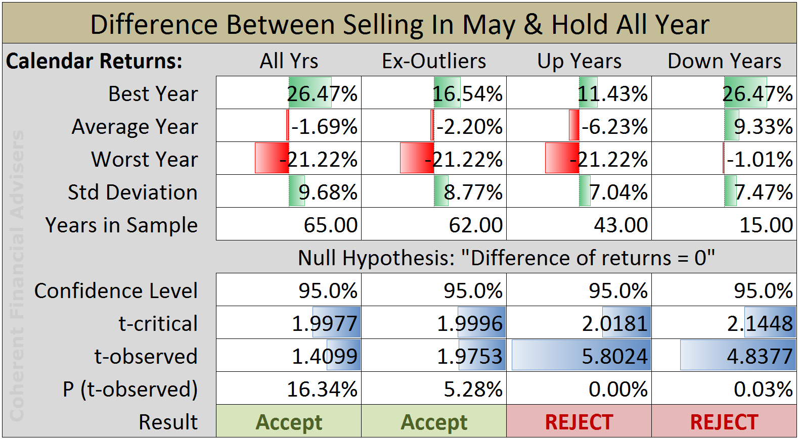
The average difference in calendar year performance between selling in May and holding all months depends on whether the year is up or down. Selling in May during up years underperforms on average by more than 6% per year. Conversely, selling in May during down years outperforms on average by more than 9% per year. The chance of either of these differences being random is virtually zero according to their respective P-values.

“Investing has always depended on knowing what is the trend now, and what is its likelihood of changing in the near term.”

Question #3: How Would My Portfolio Have Perform If I Sat In Cash May Through October?

Not as well. The following chart (figure-5) tracks the value of two $10,000 equity portfolios, one invested all months, and the other in cash from May through October. The black line is the cumulative performance difference starting 1951. By the end of 2015, the sell in May portfolio is behind by about $400,000.

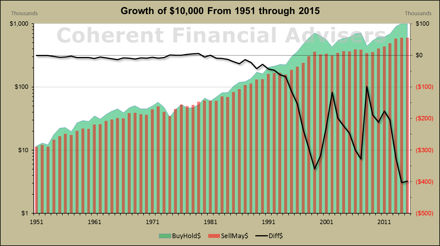
This again confirms what we know from our box plot and hypothesis testing. Selling in May benefits in years that the market is down. Our sell in May portfolio underperformed² sharply during bull markets such as in 1994, 2002 and 2009. It outperformed even more in bear markets as in 2000 and 2008.

“In my experience there is one Wall Street saying which truly makes sense, ’The trend is your friend.’”

The Bottom Line On Selling In May

Blindly selling in May underperforms on average, but significantly outperforms in down years. The only constant benefit is less volatility. The real answer is that it depends on the market’s trend. In my experience there is one Wall Street saying which truly makes sense, “The trend is your friend.”

At Coherent, we employ a diverse arsenal of rational and effective tools, research, and methodologies aimed at mitigating market risk. We are not married to only one philosophy, but bring all we know to bear according to each situation to best serve our clients. We never stop learning.

If you have any questions or comments, we would be delighted to hear from you.

 
Warm regards,
Sargon Zia, CFA
May 30, 2016

You are welcome to comment!

Recommended Reading:
What Moves The Market?
Coherent Investor September 2016
…other posts on seasonality

Footnotes:

1. We use “accept” as an abbreviation for the more proper terminology, “fail to reject”.
2. This relationship is more easily seen in the right side of the chart due to the compounding effect, and the right scale being linear rather than geometric. Selected sample period will affect results, but on average selling in May outperforms mainly in down markets.

Our Study’s Methodology:

• For this article, we abridged our research to the U.S. stock market as represented by the S&P 500 Price Index for the 65 years from 1951 through 2015. We disregarded the effects of arbitrage, dividends, taxes and transaction fees on performance, factors which are extraneous and exogenous to the basic questions at hand.
• To answer question-1, we performed a hypothesis test concerning the difference between means of dependent samples. The null hypothesis is that there is no difference. We removed calendar years in which full year return fell was outside the 95% normal probability distribution (excluded +/-2.5% tails), namely 1954, 1974, and 2008. We performed the classical approach at the standard 5% significance level using William S. Gosset’s “Student’s t” distribution. We also supplied the P-value or probability for the observed t-scores to quantify the chance of a false positive.
• To answer question-2, we used all 65 years of data without exclusions, segregated into up and down years. To distinguish between up and down years using something other than zero, we designated returns within a band of 2.5% probability on either side of zero as “flat” years, assuming an approximately normal distribution.
• To answer question-3, we invested $10,000 in each scenario, one invested all months while the other went to cash at 0% interest from May through October. We tracked the value of each portfolio for the entire 65-year sample and calculated the cumulative difference.

Print PDF